%%capture
# Setup
import emzed
import os

# path to files
data_folder = os.path.join(os.getcwd(), "tutorial_data")
path_aa_peaks_table = os.path.join(data_folder, "amino_acids_table.csv")
path_pm_aa_std = os.path.join(data_folder, "AA_std_5uM.mzML")
path_sample_caulobacter = os.path.join(data_folder, "AA_sample_caulobacter.mzML")
path_sample_arabidopsis = os.path.join(data_folder, "AA_sample_arabidopsis.mzML")
2 First steps: a targeted analysis example
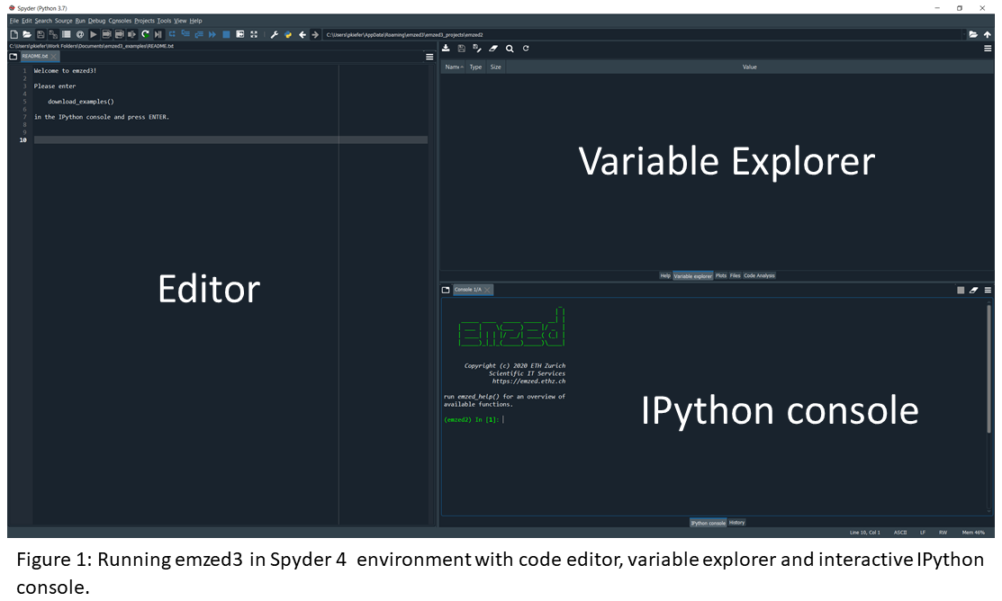
In this section, we will introduce some basic emzed features and data types required to perform a simple targeted workflow. The given example uses LC-MS measurements of proteinogenic amino acids ([M+H]+ ions) with an LTQ-Orbitrap instrument. It comprises a standard mixture containing 17 amino acids, and extracts of the two model organisms Arabidopsis thaliana and Caulobacter crescentus.
Goals
- Getting familiar with the emzed environment
- First steps with emzed core data structures PeakMap and Table
- First steps with emzed modules
- Learning how to load, visualize and inspect raw data -> the peak map
- Getting familiar with the iPython console
- Basic operations with emzed Table
- First steps with the editor
- Using simple functions to structure workflow code
emzed namespace
Everything starts with emzed.*

In the IPython console, you can directly access the emzed3 modules and its commands. All emzed functionalities are directly accessible.
Here is a short overview of the emzed modules:
align: aligning retention time, m/z and samplesadducts: provides adduct informationannotate:** features adduct annotationext: accessing downloadableemzedextensions (i.e. mzmine2)db: provides integrated pubchem databasechemistry: provides chemical informationgui: provides predefined user dialogsio: load and save datams2: supports simplified data accessquantification: allows LC-MS peak integrationtargeted: features targeted peaks extraction
An example: To obtain a list of single charged adducts in the positive mode, execute the command:
emzed.adducts.positive_single_charged
| id | adduct_name | m_multiplier | adduct_add | adduct_sub | z | sign_z |
|---|---|---|---|---|---|---|
| int | str | int | str | str | int | int |
| 19 | M+ | 1 | 1 | 1 | ||
| 20 | M+H | 1 | H | 1 | 1 | |
| 21 | M+NH4 | 1 | NH4 | 1 | 1 | |
| 22 | M+Na | 1 | Na | 1 | 1 | |
| 23 | M+H-2H2O | 1 | H | (H2O)2 | 1 | 1 |
| 24 | M+H-H2O | 1 | H | H2O | 1 | 1 |
| 25 | M+K | 1 | K | 1 | 1 | |
| 26 | M+ACN+H | 1 | C2H3NH | 1 | 1 | |
| 27 | M+2ACN+H | 1 | (C2H3N)2H | 1 | 1 | |
| 28 | M+ACN+Na | 1 | (C2H3N)1Na | 1 | 1 | |
| 29 | M+2Na-H | 1 | Na2 | H | 1 | 1 |
| 30 | M+Li | 1 | Li | 1 | 1 | |
| 31 | M+CH3OH+H | 1 | CH3OHH | 1 | 1 | |
| 32 | M+2K-H | 1 | K2 | H | 1 | 1 |
| 33 | M+IsoProp+H | 1 | (C3H8O)1H | 1 | 1 | |
| 34 | M+IsoProp+Na+H | 1 | (C3H8O)1NaH | 1 | 1 | |
| 35 | M+DMSO+H | 1 | (C2H6OS)1H | 1 | 1 | |
| 36 | 2M+H | 2 | H | 1 | 1 | |
| 37 | 2M+NH4 | 2 | NH4 | 1 | 1 | |
| 38 | 2M+Na | 2 | Na | 1 | 1 | |
| 39 | 2M+K | 2 | K | 1 | 1 | |
| 40 | 2M+ACN+H | 2 | (C2H3N)1H | 1 | 1 | |
| 41 | 2M+ACN+Na | 2 | (C2H3N)1Na | 1 | 1 |
Note: In the IPython console you can directly access the command documentation (docstring) by adding a ? at the end.
Inspecting raw data
To inspect raw data (mzML, mzXML files) two commands are required:
pm = emzed.io.load_peak_map()
emzed.gui.inspect(pm)
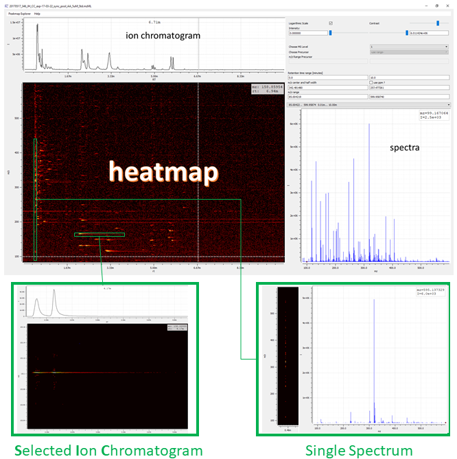
Figure 2: Visualizing the raw data of an example file. emzed peak map explorer provides data visualization as heat map with retention time values (RT) on x-axis and m/z values on y-axis, corresponding total ion chromatogram (TIC, sum of all m/z peaks), and the overlay of all m/z spectra.
The output is an emzed Table containing all information required to determine the corresponding molecular mass of an adduct ion.
Peak extraction with emzed Table
Table is the core data structure of emzed. It appears as typical table with rows and columns. If you are familiar with pandas data frames you will see some similar properties. Each column has a unique name shown in the first row and contains values of a defined data types. In the following we will use Table to visualize peaks of LC-MS raw data measurements.
We will start by loading a csv file containing mz data of selected amino acids as Table. Note, it is possible to save Tables as and load Tables from CSV and XLS(X) files enabling straightforward creation of tables for targeted peaks extraction.
aa_peaks_table = emzed.io.load_csv(
    path_aa_peaks_table
)  # we provide the path of .csv file...
# Without arguments a user dialog will open.
aa_peaks_table[:5]  # list indexing on table rows
| compound | mf | m0 | mz |
|---|---|---|---|
| str | str | float | MzType |
| Phenylalanine | C9H11NO2 | 165.079000 | 166.086300 |
| Leucine | C6H13NO2 | 131.094600 | 132.101900 |
| Tryptophane | C11H12N2O2 | 204.089900 | 205.097200 |
| Isoleucine | C6H13NO2 | 131.094600 | 132.101900 |
| Methionine | C5H11NO2S | 149.051100 | 150.058300 |
When printing the table, you get name, type and the formatted content of each table column. In our case we have columns of types int, str, and float. Concerning column names there are two different groups: predefined column names and user defined. Predefined columns have fixed names, types, formats and they are required for most Table operations with MS data.
You can find a complete list of predefined column names here
More general information about the Table is available via the command:
aa_peaks_table.summary()
| id | name | type | format | nones | len | min | max | distinct values |
|---|---|---|---|---|---|---|---|---|
| int | str | str | str | int | int | float | float | int |
| 0 | compound | str | %s | 0 | 21 | - | - | 21 |
| 1 | mf | str | %s | 0 | 21 | - | - | 19 |
| 2 | m0 | float | %f | 0 | 21 | 75.032000 | 204.089900 | 19 |
| 3 | mz | MzType | %11.6f | 0 | 21 | 76.039300 | 205.097200 | 19 |
For each column the command provides content information i.e. name, type, format.
We can use now given table to inspect the amino acid peaks of our standard file.
To visualize LC-MS peaks a Table requires the columns id, mzmin, mzmax, rtmin, rtmax, and peakmap.
These columns are used to define the LC-MS peaks that will later be extracted and integrated. mzmin and mzmax are the lower and upper bounds of the mz values, while rtmin and rtmax define the retention time boundaries of the peak. The peakmap column contains the LC-MS peak map, i.e. the raw data.
We will use Table method add_column to add those columns to aa_table:
aa_peaks_table.add_column("mzmin", aa_peaks_table.mz - 0.003, emzed.MzType)
aa_peaks_table.add_column("mzmax", aa_peaks_table.mz + 0.003, emzed.MzType)
add_column requires three arguments: column name, the values you want to add, and the value type. In the given example we add a new column mzmin using existing column mz:
aa.mz - 0.003
Hence, we take the values of column mz in table aa and subtract 0.003. In other words, we can directly perform operations on columns. Note, it is mandatory to define the argument type_! Also note, rt and mz columns have a specific emzed type.
Next, we have to add the columns rtmin and rtmax. Currently, we do not know the retention times (RT) of the different amino acid peaks. One way to access RTs is inspecting again the peak map and then manually extract the values. For now, we will just set rtmin and rtmax such that they cover the entire length of the run. To do so, we first load the PeakMap object with:
# we load the peakmap from path path_aa_std
peakmap_std = emzed.io.load_peak_map(path_pm_aa_std)
Similar to Table, PeakMap provides a multitude of methods. The PeakMap method rt_range() returns a tuple with the first value corresponding to the RT of the first measured spectrum and the second to the last. Please note that RT values are given in seconds. We can extract rtmin and rtmax by the command:
rtmin, rtmax = peakmap_std.rt_range()
print(f"rtmin = {rtmin}, rtmax = {rtmax}")
rtmin = 0.3225, rtmax = 599.8278
Now we can add the columns rtmin and rtmax to the table:
aa_peaks_table.add_column_with_constant_value("rtmin", rtmin, emzed.RtType)
aa_peaks_table.add_column_with_constant_value("rtmax", rtmax, emzed.RtType)
You might have realized, that we used the method add_column_with_constant_value since Table distinguish between an iterable with potential different row values and a constant value, respectively. Ignoring the difference will cause an error.
Next, we have to add the peak map to the table:
aa_peaks_table.add_column_with_constant_value("peakmap", peakmap_std, emzed.PeakMap)
Finally the column id, providing unique row identification values, is added:
aa_peaks_table.add_enumeration()
aa_peaks_table[:10] # or aa_table.print_(max_rows=10)
| id | compound | mf | m0 | mz | mzmin | mzmax | rtmin | rtmax |
|---|---|---|---|---|---|---|---|---|
| int | str | str | float | MzType | MzType | MzType | RtType | RtType |
| 0 | Phenylalanine | C9H11NO2 | 165.079000 | 166.086300 | 166.083300 | 166.089300 | 0.01 m | 10.00 m |
| 1 | Leucine | C6H13NO2 | 131.094600 | 132.101900 | 132.098900 | 132.104900 | 0.01 m | 10.00 m |
| 2 | Tryptophane | C11H12N2O2 | 204.089900 | 205.097200 | 205.094200 | 205.100200 | 0.01 m | 10.00 m |
| 3 | Isoleucine | C6H13NO2 | 131.094600 | 132.101900 | 132.098900 | 132.104900 | 0.01 m | 10.00 m |
| 4 | Methionine | C5H11NO2S | 149.051100 | 150.058300 | 150.055300 | 150.061300 | 0.01 m | 10.00 m |
| 5 | Valine | C5H11NO2 | 117.079000 | 118.086300 | 118.083300 | 118.089300 | 0.01 m | 10.00 m |
| 6 | Proline | C5H9NO2 | 115.063300 | 116.070600 | 116.067600 | 116.073600 | 0.01 m | 10.00 m |
| 7 | Tyrosine | C9H11NO3 | 181.073900 | 182.081200 | 182.078200 | 182.084200 | 0.01 m | 10.00 m |
| 8 | Cysteine | C3H7NO2S | 121.019700 | 122.027000 | 122.024000 | 122.030000 | 0.01 m | 10.00 m |
| 9 | Alanine | C3H7NO2 | 89.047700 | 90.055000 | 90.052000 | 90.058000 | 0.01 m | 10.00 m |
aa_peaks_table.summary()
| id | name | type | format | nones | len | min | max | distinct values |
|---|---|---|---|---|---|---|---|---|
| int | str | str | str | int | int | float | float | int |
| 0 | id | int | %d | 0 | 21 | 0.000000 | 20.000000 | 21 |
| 1 | compound | str | %s | 0 | 21 | - | - | 21 |
| 2 | mf | str | %s | 0 | 21 | - | - | 19 |
| 3 | m0 | float | %f | 0 | 21 | 75.032000 | 204.089900 | 19 |
| 4 | mz | MzType | %11.6f | 0 | 21 | 76.039300 | 205.097200 | 19 |
| 5 | mzmin | MzType | %11.6f | 0 | 21 | 76.036300 | 205.094200 | 19 |
| 6 | mzmax | MzType | %11.6f | 0 | 21 | 76.042300 | 205.100200 | 19 |
| 7 | rtmin | RtType | rt_formatter | 0 | 21 | 0.322500 | 0.322500 | 1 |
| 8 | rtmax | RtType | rt_formatter | 0 | 21 | 599.827800 | 599.827800 | 1 |
| 9 | peakmap | PeakMap | None | 0 | 21 | - | - | 1 |
Now the table is ready for inspection. Just type:
emzed.gui.inspect(aa_peaks_table)
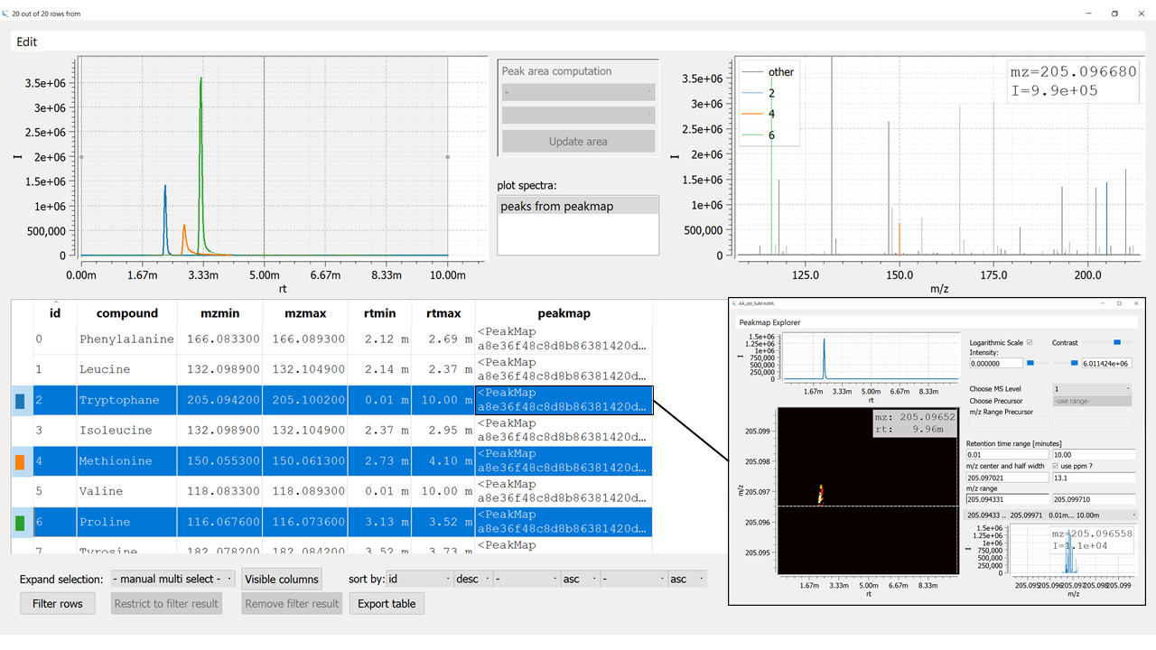 Figure 2: Visualization of an emzed Table using the Table Explorer. The inset on the bottom right shows the Peakmap Explorer that opens up after double clicking an entry in the column
 peakmap.
Some comments
LC-MS Peaks Tables require columns with fixed names and types.
Required columns
mz,mzmin,mzmax,rtmin,rtmaxandpeakmaphave emzed specific types, which can be directly accessed viaemzed.MzTypeandemzed.RtType. They come along with special formatting. In particular, rt values are given in seconds, but shown in minutes.The column
peakmapallows keeping track to the raw data.
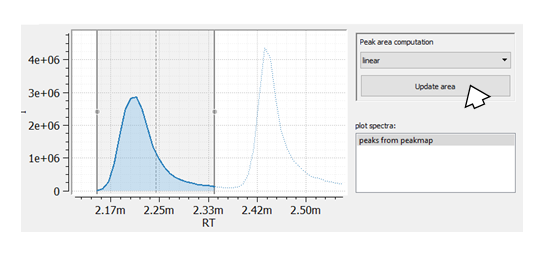
Defining EIC-peaks. Since we did not yet define the accurate retention time (RT) window, each row shows the complete EIC of the corresponding amino acid. The easiest way to adapt the RT windows is using the emzed integrate method, which not only calculates the peak area but also features interactive definition of RT windows. Until now, we applied only Table methods like i.e. add_column operating in place, meaning the method modifies the table but does not create a new Table object. This is memory efficient because we do not have to copy the object after each operation. integrate is not a Table method and will return a new objectby default. We will first explore how to integrate:
emzed.quantification.integrate(peak_table, peak_shape_model)
The function integrate requires the two mandatory arguments peak_table and peak_shape_model.
Available peak integration models are: linear, sgolay, no_integration, asym_gauss emg, and emg_robust. The two models linear and sgolay are both using trapezoidal rule as numerical approximation method and do not assume a defined peak shape. The sgolay method includes noise filtering step prior to integration. In contrast, asym_gauss and emg_exact model are assuming distinct, Gaussian-related distributions. Last but not least, no_integration returns None as the area. Note, integrate has a large number of optional predefined arguments that we can simply keep as they are and that we will discuss later. Hence, we can integrate aa_table as follows:
aa_peaks_table = emzed.quantification.integrate(
    aa_peaks_table, "linear", show_progress=False
)
aa_peaks_table.summary()
| id | name | type | format | nones | len | min | max | distinct values |
|---|---|---|---|---|---|---|---|---|
| int | str | str | str | int | int | float | float | int |
| 0 | id | int | %d | 0 | 21 | 0.000000 | 20.000000 | 21 |
| 1 | compound | str | %s | 0 | 21 | - | - | 21 |
| 2 | mf | str | %s | 0 | 21 | - | - | 19 |
| 3 | m0 | float | %f | 0 | 21 | 75.032000 | 204.089900 | 19 |
| 4 | mz | MzType | %11.6f | 0 | 21 | 76.039300 | 205.097200 | 19 |
| 5 | mzmin | MzType | %11.6f | 0 | 21 | 76.036300 | 205.094200 | 19 |
| 6 | mzmax | MzType | %11.6f | 0 | 21 | 76.042300 | 205.100200 | 19 |
| 7 | rtmin | RtType | rt_formatter | 0 | 21 | 0.322500 | 0.322500 | 1 |
| 8 | rtmax | RtType | rt_formatter | 0 | 21 | 599.827800 | 599.827800 | 1 |
| 9 | peakmap | PeakMap | None | 0 | 21 | - | - | 1 |
| 10 | peak_shape_model | str | %s | 0 | 21 | - | - | 1 |
| 11 | area | float | %.2e | 0 | 21 | 0.000000 | 27402460.271635 | 19 |
| 12 | rmse | float | %.2e | 0 | 21 | 0.000000 | 0.000000 | 1 |
| 13 | model | object | None | 0 | 21 | - | - | 19 |
| 14 | valid_model | bool | bool_formatter | 0 | 21 | - | - | 1 |
The function integrate adds 5 additional columns to the table. the columns area and rmse are showing peak area and the mean root square error (rmse) of the area. The latter describes the rmse of the selected model named column peak_shape_model in comparison with the linear model as reference. For each peaks, the column model contains ab object with its individual integration parameters. Finally, the column valid_model is internal and can be ignored.
After integration, inspecting the resulting Table t gives:
emzed.gui.inspect(aa_peaks_table)
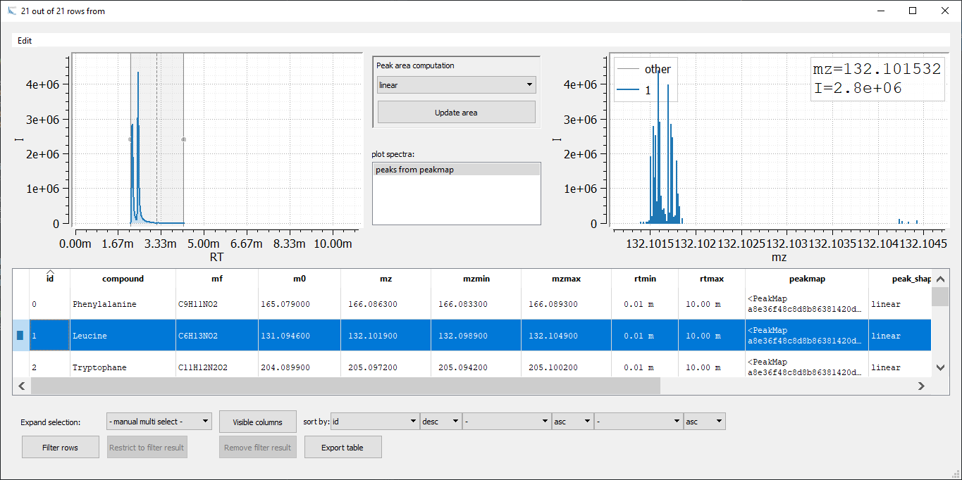
Now, we are able to adapt the RT window width for each peak manually: We change the peak window boarders with the mouse and we adapt rtmin and rtmax by simply reintegrating the peak (pressing the Update area button).
Summarized. With the two Table methods add_column and add_column_with_constant_value we could build an emzed Table that allows extracting and visualizing EICs from a raw data file using a predefined list of compounds given as .csv file. We can use the function integrate and the interactive Table explorer to manually select peaks within EICs resulting in a peak table containing individual RT/mz windows for all peaks.
Simple scripts
It is quite cumbersome to execute required commands one by one in the IPython console and organizing the commands in a script is a much better way to proceed. The easiest way to do so is writing all the command we have executed so far into a Python script. Spyder provides a history log showing us all commands we executed so far.
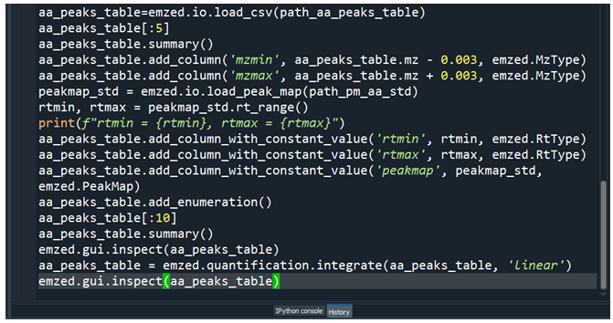
We can proceed by simply copy paste the commands shown in history log into the editor and remove all commands that are not required. We end up with a script similar to the following:
import emzed

# loading data
peakmap_std = emzed.io.load_peak_map()
aa_peaks_table = emzed.io.load_csv()

# creating peaks table
rtmin, rtmax = peakmap_std.rt_range()

aa_peaks_table.add_column('mzmin', aa_peaks_table.mz - 0.003, emzed.MzType)
aa_peaks_table.add_column('mzmax', aa_peaks_table.mz + 0.003, emzed.MzType)
aa_peaks_table.add_column_with_constant_value('rtmin', rtmin, emzed.RtType)
aa_peaks_table.add_column_with_constant_value('rtmax', rtmax, emzed.RtType)
aa_peaks_table.add_column_with_constant_value('peakmap', peakmap_std, emzed.PeakMap)
aa_peaks_table.add_enumeration()

# integrate peaks table
aa_peaks_table = emzed.quantification.integrate(aa_peaks_table, 'linear')

# adapt retention of peaks manually
emzed.gui.inspect(aa_peaks_table)
You can execute the code by pressing F5. When executing the script for the first time a cofiguration window will pop up. Just press the window ok button and the script gets executed.
There are several disadvantages of direct code execution. Since all intermediate results end up in the workspace, longer scripts can provoke messy workspaces. Code readability counts: Long unstructured scripts are hard to understand in particular, when the workflow is not a linear sequence of commands. Finally, you cannot execute only parts of the script and each time you have to run the complete script. To increase code reproducibility we can organize functional blocks of our scripts into Pythin functions, i.e. a function building a peaks_table that allow manual RT window definition:
def build_peak_table(t, peakmap, mztol=0.003):
    """builds table defining EICs inspectable in peakmap
    t: Table with required column `mz`
    peakmap: emzed PeakMap
    """
    t.add_column("mzmin", t.mz - mztol, emzed.MzType)
    t.add_column("mzmax", t.mz + mztol, emzed.MzType)
    rtmin, rtmax = peakmap_std.rt_range()
    t.add_column_with_constant_value("rtmin", rtmin, emzed.RtType)
    t.add_column_with_constant_value("rtmax", rtmax, emzed.RtType)
    t.add_enumeration()
    return emzed.quantification.integrate(t, "linear")
We can load the function by pressing again F5 and it is available in the IPython console.
Batch extraction of amino acids. The sample containing amino acid standards allowed us to define the amino acid peaks via mzmin, mzmax, rtmin, rtmax. To perform a targeted extraction of amino acid peaks from other samples, we simply have to replace the peak map of the standard in the peaks table, by the sample peak map, and reintegrate the table. Since the method replace operates in place we would modify our peaks with each extraction and the original peak map containing the standards will get lost. To avoid this we will create a copy of aa_peak_table.
peak_table = aa_peaks_table.copy()
sample = emzed.io.load_peak_map(path_sample_caulobacter)
peak_table.replace_column_with_constant_value("peakmap", sample, emzed.PeakMap)
t_sample = emzed.quantification.integrate(peak_table, "linear", show_progress=False)
Let's inspect the resulting Table t_sample:

For a greater number of samples it makes sense to write a little routine to extract amino acids from a batch of samples that could look like this:
def extract_peaks(peak_table, peakmap_sample):
    pt = peak_table.copy()
    pt.replace_column_with_constant_value('peakmap', peakmap_sample, emzed.PeakMap)
    return emzed.quantification.integrate(pt, 'linear')

# load peak table
peak_table = emzed.io.load_table()

# load sample batch
samples = emzed.io.load_peak_maps()

# extract peaks from all samples with Python list comprehension
results = [extract_peaks(peak_table, sample) for sample in samples]

# To inspect peak extraction result use list indexing (i.e. last sample):
emzed.gui.inspect(results[-1])