%%capture
# Setup
import emzed
import os

# path to files
data_folder = os.path.join(os.getcwd(), "tutorial_data")
path_table_caulobacter = os.path.join(data_folder, "t_caulo_ffmetabo.table")
path_table_arabidopsis = os.path.join(data_folder, "t_ara_ffmetabo.table")
ref_path = os.path.join(data_folder, "mz_calibration_table.csv")
t_caulo = emzed.io.load_table(path_table_caulobacter)
t_ara = emzed.io.load_table(path_table_arabidopsis)
t_ref = emzed.io.load_csv(ref_path)
6 Alignment
The emzed3 alignment module provides functions that allow correcting for instrument drifts (mz, RT), which occurred during data acquisition. Note, all alignment processes operate on LC-MS peak level and a preceding peak detection step is required.
Retention time alignment
There are multiple reasons (e.g. sample matrix, variation in buffer composition) provoking retention time shifts between samples analyzed with the same LC-MS method. Depending on the observed retention time differences, aligning can enhance the mapping of identical peaks in different samples significantly, as the required retention time tolerance can be reduced. In principle, the algorithm maps peaks of a reference table and a feature table with similar mz values and within a user defined retention time window. Based on peak mapping, a function $\Delta RT(RT)$ is created and a curve fit is applied to the curve. Subsequently, the retention time of each spectrum in the peak map is shifted as a function of the fit curve. Hence, the quality of retention time shift depends a lot on the number of correct peak mappings and on the applied fitting.
In emzed, the emzed.align.rt_align function is used for RT alignment. The algorithm originates from OpenMS and you can find some information about it here. RT alignment in emzed requires the specific column names feature_id, rt, mz, and intensity present in run_feature_finder_metabo output tables. If you want to align peak tables generated with the mzmine2 extension, you have to rename column names accordingly!
The emzed.align.rt_align function has a number of arguments that require some explanations:
rt_align(tables, reference_table=None, destination=None, reset_integration=False, n_peaks=-1, max_rt_difference=100, max_mz_difference=0.3, max_mz_difference_pair_finder=0.5, model='b_spline', **model_parameters)
tables: A list of feature tables created with e.g. run_feature_finder_metabo.reference_table: Extra reference table, if None the table with most features among tables is taken. A reference Table is in particular useful when using a global reference for routine measurements. Aligning all your measurements to the same table significantly enhances long term sample comparison over different batches. Note, a significant peak overlap between reference_table and tables is required for good retention time alignment.destination: Target folder for quality plots $\Delta RT(RT)$ including the fitting curve (see Figure below). For each feature table a quality plot is created. Such plots are in particular useful for parameter tuning (e.g. checking whether the reference table is suitable).reset_integration: Sets all column values related to integration (i.e. area) toNoneif present. Else the alignment will fail for already integrated tables. Why resetting peak integration? Because changing the rt values of spectra can have an influence on peak boundaries, meaning the peak areas are no longer correct. If possible, do integrate peaks after retention time alignment!n_peaks: The maximal number of peaks matched by matching algorithm, where -1 means all peaks. The value can be a float between 0 and 1 to refer to the fraction of peaks in reference table. Peaks are selected by their intensity. In general, the default value of -1 works well.max_rt_difference: Max allowed difference of rt values in seconds for searching matching features. The value should be adapted to the data set. An overestimation will significantly lower the alignment quality.max_mz_difference_pair_finder: Max allowed difference in mz values for pair finding.model: The two available fitting models are b-spline and lowess. Both fitting models can be adapted to obtain good fitting results since lowess allows using cubic spline as fitting function. However, b-spline applies least square, whereas lowess uses weighted least square for error minimization. Hence, when applying lowess, data points closer to the fitting will be weighted stronger, which makes the approach less sensitive to outliers and should be advantageous with more noisy data.model_parameters: Keyword parameters depending on provided value formodel.model='b_spline'num_nodes: Number of break points of fitted spline (default: 5). Note, that more points result in splines with higher variation and thatnum_nodesmust be uneven.
model='lowess'span: Value between 0 and 1, larger values lead to more smoothing (default is 2/3). The smaller the value the more local regression segments will be defined.interpolation_type: either"cspline"or"linear"(default:"linear")
Again, we will use the Arabidopsis and Caulobacter cell extract samples to demonstrate RT alignment. The two examples originate from two different batches. We can observe a significant retention time shift increasing with increasing retention time (see Figure 6 below).
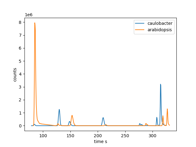
Figure 6. Selected peaks from Caulobacter (left peak) and Arabidopsis (right peak) samples to demonstrate the retention time shift.
We can observe a maximal retention time shift for late eluting peaks of about 10 s. Since the number of common peaks of the two example files is low, we can extract all peaks used for the alignment process by a simple join with max_rt_difference = 10 as absolute RT tolerance and max_mz_pair_difference = 0.005 as absolute mz tolerance:
max_mz_pair_difference = 0.005
max_rt_difference = 10
mz_condition = t_caulo.mz.approx_equal(t_ara.mz, max_mz_pair_difference, 0)
rt_condition = t_caulo.rt.in_range(
    t_ara.rt - max_rt_difference, t_ara.rt + max_rt_difference
)
t_common = t_caulo.join(t_ara, mz_condition & rt_condition)
print(f"number of common peaks: {len(t_common)}")
number of common peaks: 17
import matplotlib.pyplot as plt

# we calculate the delta rt
t_common.add_or_replace_column("delta_rt", t_common.rt - t_common.rt__0, float)
rt = t_common.rt.to_list()
delta_rt = t_common.delta_rt.to_list()
plt.plot(rt, delta_rt, "*")
plt.xlabel("Retention time (s)")
plt.ylabel(r"$\Delta$ RT (s)")
plt.show()

The plot indicates a more or less linear retention time difference decrease. We can now apply the RT alignment function using the two different fitting models with default fitting model settings and check the fitting quality.
rt_align = emzed.align.rt_align
tables = [t_caulo, t_ara]
tables_spline = rt_align(
    tables,
    max_rt_difference=20.0,
    max_mz_difference=0.005,
    max_mz_difference_pair_finder=0.005,
)  # default model is b-spline
tables_lowess = rt_align(
    tables,
    max_rt_difference=20.0,
    max_mz_difference=0.005,
    max_mz_difference_pair_finder=0.005,
    model="lowess",
)
reference_map is <noname>
pyopenms: Progress of 'affine pose clustering':
pyopenms:
pyopenms: -- done [took 0.00 s (CPU), 0.00 s (Wall)] --
reference_map is <noname>
pyopenms: Progress of 'affine pose clustering':
pyopenms:
pyopenms: -- done [took 0.00 s (CPU), 0.00 s (Wall)] --
Alignment results:
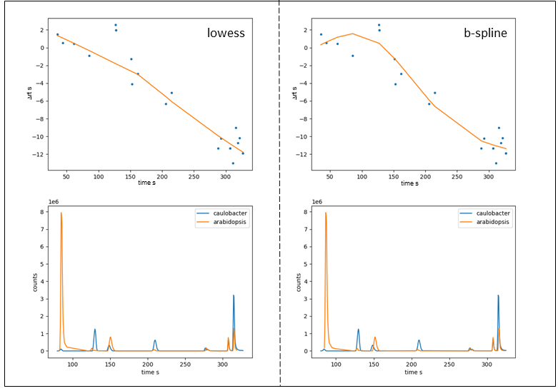
Figure 7: Fitting curve (top) and selected LC-MS peaks of aligned samples (bottom) after RT alignment obtained with lowess (left) and b-spline (right).
For the given example, lowess results in a slightly better alignment. However, as already mentioned, the two samples have very few peaks in common meaning choosing the default number of nodes for b-spline fitting (5) tends to overfit. When reducing the number of nodes to 3 we obtain fitting results very similar to those obtained with lowess. Analogous, we can drastically reduce the robustness of the lowess fit by lowering the span value from 0.66 to 0.3 thus increasing the local weights drastically, which is similar to increasing num_nodes with b_spline fit.

Figure 8: Fitting curve (top) and selected LC-MS peaks of aligned samples (bottom) after RT alignment. $RT$ vs $\Delta RT$ plots of b_spline fit with num_nodes = 7 and lowess fit with span = 0.3.
The given example with very few peaks in common was selected to simplify the demonstration of fit models and corresponding parameters. Typically, the number of common peaks is much higher as shown in Figure 9.
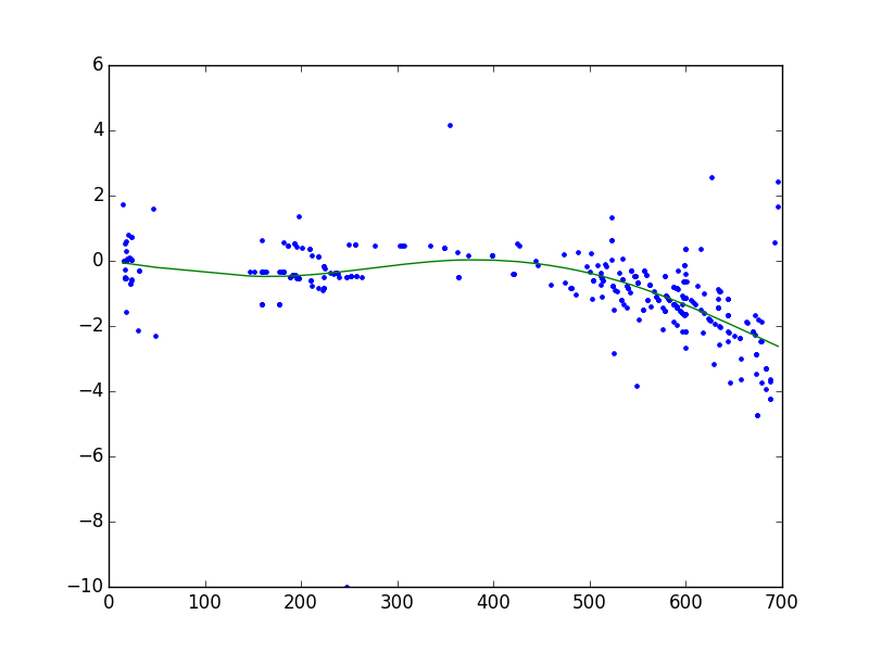
Figure 9: Typical retention time alignment using default fit model settings ("b-spline" , num_nodes = 5)
m/z alignment
emzed3 provides the possibility to perform a "post acquisition mass calibration" based on known m/z peaks to correct for m/z instrument drifts. The mass accuracy stability depends on the type of intrument and can vary more or less significantly over time and noticeable mass drifts might be observed.
t_aligned = mz_align(table, reference_table, tol=0.015, destination=None, min_r2=0.95, max_tol=0.001, min_points=5, interactive=False)
The functions performs affine linear mz value correction for feature tables with function arguments
table: a peaks table with required columnsreference table: Table defining reference peaks with required the columnsnamecompound namesmzcalculated mz values of compoundsrtmin,rtmax, the expected retention time windowpolaritythe polarity of the compound ion (+/-)
tol: maximal tolerated difference of reference and feature table mz values to include compound peak into fitting procsess.destination: Target folder for quality plots $\Delta RT(RT)$ including the fitting curve (see Figure 7). For each feature table a quality plot is created.min_r2: Minimal quality of linear regression. Fitting results with $R^{2} < min_r2$ will be ignored.max_tol: maximal allowed m/z diffence between calculated and corrected m/z values. Fitting results containing calibration peaks with $abs(mz_corr-mz_calc) > max$ will be ignored.interactive: The interactive mode allows peak exclusion from the fitting curve by the user.
In chapter 3 we extracted amino acids by a targeted approach. We can use amino acid peaks to demonstrate mz alignment.
t_ref
| name | mf | m0 | mz | rt | rtmin | rtmax | polarity |
|---|---|---|---|---|---|---|---|
| str | str | float | MzType | RtType | RtType | RtType | str |
| Phenylalanine | C9H11NO2 | 165.079000 | 166.086300 | 2.27 m | 2.14 m | 2.40 m | + |
| Leucine | C6H13NO2 | 131.094600 | 132.101900 | 1.65 m | 1.52 m | 1.78 m | + |
| Tryptophane | C11H12N2O2 | 204.089900 | 205.097200 | 2.35 m | 2.22 m | 2.48 m | + |
| Valine | C5H11NO2 | 117.079000 | 118.086300 | 3.27 m | 3.14 m | 3.40 m | + |
| Tyrosine | C9H11NO3 | 181.073900 | 182.081200 | 3.63 m | 3.50 m | 3.76 m | + |
| Alanine | C3H7NO2 | 89.047700 | 90.055000 | 4.00 m | 3.87 m | 4.13 m | + |
| Threonine | C4H9NO3 | 119.058200 | 120.065500 | 4.61 m | 4.48 m | 4.74 m | + |
mz_align = emzed.align.mz_align
t_mz_aligned = mz_align(t_caulo, t_ref)
t1 = t_caulo.extract_columns("id", "mz")
t2 = t_mz_aligned.extract_columns("id", "mz")
comp = t1.join(t2, t1.id == t2.id)
comp[10:100:10]
5 MATCHES FROM REFERENCE
NUMPOINTS=  5  goodness=0.014
| id | mz | id__0 | mz__0 |
|---|---|---|---|
| int | MzType | int | MzType |
| 10 | 104.070310 | 10 | 104.070613 |
| 20 | 112.075332 | 20 | 112.075635 |
| 30 | 118.085986 | 30 | 118.086289 |
| 40 | 128.106696 | 40 | 128.106997 |
| 50 | 132.101695 | 50 | 132.101996 |
| 60 | 141.102055 | 60 | 141.102356 |
| 70 | 148.060255 | 70 | 148.060555 |
| 80 | 151.122885 | 80 | 151.123185 |
| 90 | 153.102109 | 90 | 153.102408 |
comp[-101:-1:10]
| id | mz | id__0 | mz__0 |
|---|---|---|---|
| int | MzType | int | MzType |
| 1048 | 554.857002 | 1048 | 554.857275 |
| 1058 | 562.352317 | 1058 | 562.352589 |
| 1068 | 564.358909 | 1068 | 564.359182 |
| 1078 | 570.005582 | 1078 | 570.005854 |
| 1088 | 577.371586 | 1088 | 577.371858 |
| 1098 | 578.038838 | 1098 | 578.039109 |
| 1108 | 584.379706 | 1108 | 584.379977 |
| 1118 | 586.377630 | 1118 | 586.377901 |
| 1128 | 591.373498 | 1128 | 591.373769 |
| 1138 | 592.891840 | 1138 | 592.892110 |
Comments:
- The instrument was already well calibrated and hence we obtain a neglectable mz correction in the sub milli mass unit range.
- Selected calibration peaks are not ideal, since they do not span the complete mz range. Best practice would be to spike the samples with calibrants and corresponding LC-MS peaks do not overlap with sample peaks.
Peak table alignment
Comparing peaks in tables of different samples is quite cumbersome since identic peaks having different ids in different samples. So far, to compare peaks we applied the table methods join, left_join or filter. The alignment module provides the function align_peaks that assigns a global peak id to all samples of interest. Depending on observed mz and rt shifts it is recommended to perform rt and mz alignment prior to peak alignment.
help(emzed.align.align_peaks)
Help on function align_peaks in module emzed.align.sample_alignment:

align_peaks(tables, mz_tol, rt_tol)
    Assigns global peak ids over samples sucht that peaks which differ by
    given tolerances are are assigned to the sampe global peak id.

    Tables are modified in-place by adding a new columns ``global_peak_id``.

    :param tables: list or tuple of peak tables with columns "id", "mz" and "rt" at
                   least.
    :param mz_tol: mz tolerance in Da.
    :param rt_tol: rt tolerance in seconds.

    :returns: None
A new id global_peak_id is assigned to all tables in place. Required table column names are id, mz, rt. Depending on observed retention time and m/z shift of the data set, retention time and mass alignment should be performed prior to peak aligning. As an example we apply align_peaks to retetion time aligned samples tables_lowess:
emzed.align.align_peaks(tables_lowess, mz_tol=0.001, rt_tol=2.0)
t_all = emzed.Table.stack_tables(tables_lowess).sort_by("global_peak_id")
t_all[:10]
number of total peaks     : 1600
pyopenms: Progress of 'Linking features':
pyopenms:
pyopenms: -- done [took 0.01 s (CPU), 0.01 s (Wall)] --number of global peaks ids: 1583
| id | global_peak_id | feature_id | feature_size | mz | mzmin | mzmax | rt | rtmin | rtmax | intensity | quality | fwhm | z | source |
|---|---|---|---|---|---|---|---|---|---|---|---|---|---|---|
| int | int | int | int | MzType | MzType | MzType | RtType | RtType | RtType | float | float | RtType | int | str |
| 10 | 0 | 9 | 1 | 104.070310 | 104.070198 | 104.070457 | 2.65 m | 2.60 m | 2.73 m | 5.82e+05 | 1.31e-04 | 0.08 m | 0 | AA_sample_caulobacter.mzML |
| 1 | 0 | 1 | 1 | 104.070530 | 104.070404 | 104.070633 | 2.65 m | 2.55 m | 2.75 m | 2.93e+06 | 3.62e-03 | 0.10 m | 0 | AA_sample_arabidopsis.mzML |
| 11 | 1 | 10 | 1 | 104.106672 | 104.106583 | 104.106750 | 1.41 m | 1.36 m | 1.45 m | 2.72e+05 | 6.10e-05 | 0.05 m | 0 | AA_sample_caulobacter.mzML |
| 2 | 1 | 2 | 2 | 104.106882 | 104.106766 | 104.107101 | 1.42 m | 1.38 m | 1.94 m | 1.89e+07 | 2.40e-02 | 0.04 m | 1 | AA_sample_arabidopsis.mzML |
| 5 | 2 | 5 | 1 | 92.663911 | 92.663506 | 92.664627 | 0.89 m | 0.86 m | 1.01 m | 2.98e+05 | 6.69e-05 | 0.05 m | 0 | AA_sample_caulobacter.mzML |
| 7 | 3 | 7 | 1 | 99.091387 | 99.091187 | 99.091454 | 1.14 m | 1.11 m | 1.22 m | 1.18e+06 | 2.65e-04 | 0.04 m | 0 | AA_sample_caulobacter.mzML |
| 14 | 4 | 13 | 1 | 105.042087 | 105.041962 | 105.042160 | 3.87 m | 3.86 m | 3.89 m | 4.95e+04 | 1.11e-05 | 0.03 m | 0 | AA_sample_caulobacter.mzML |
| 8 | 5 | 8 | 2 | 102.127362 | 102.127266 | 102.127548 | 0.93 m | 0.90 m | 1.39 m | 6.95e+07 | 1.62e-02 | 0.04 m | 1 | AA_sample_caulobacter.mzML |
| 13 | 6 | 12 | 1 | 105.042006 | 105.041916 | 105.042137 | 3.56 m | 3.43 m | 3.72 m | 1.27e+06 | 2.84e-04 | 0.15 m | 0 | AA_sample_caulobacter.mzML |
| 4 | 7 | 3 | 1 | 104.106940 | 104.106728 | 104.107063 | 2.09 m | 1.95 m | 3.02 m | 5.69e+05 | 7.04e-04 | 0.20 m | 0 | AA_sample_arabidopsis.mzML |